Data drift detection: a production guide for ML engineers
Data drift detection is the practice of continuously measuring changes in the statistical distribution of input features so you can act before model quality degrades in production. According to Evidently AI, data drift is a change in the distribution of input features to a model, detectable by comparing production inputs against a reference dataset, and it often precedes measurable performance decline. The moment your production data stops resembling the data your model was trained on, every prediction it makes is extrapolating, not interpolating.
Your first three actions in any production system:
Enable univariate distribution checks on your top features by importance, using the Kolmogorov–Smirnov test for continuous variables and chi-square for categoricals.
Track your model’s score distribution daily. A shift in predicted probability histograms is often the earliest visible signal of upstream input change.
Establish a versioned reference window from a clean, representative slice of training or early production data, and lock it before you go live.
Pro Tip: Set two alert thresholds, not one: a “warning” level at a moderate PSI or KS statistic, and a “critical” level that triggers an incident. This prevents alert fatigue without letting genuine drift go unnoticed.
Key takeaways
Effective data drift detection requires monitoring input distributions and model outputs continuously, triaging alerts before retraining, and matching the response to the specific drift type detected.
Point | Details |
Monitor inputs and outputs together | Input checks give early warning; score distribution shifts confirm model impact before labels arrive. |
Use PSI and Wasserstein at scale | At large sample sizes, p-values become hypersensitive; magnitude metrics give more reliable operational signals. |
Triage before retraining | Verify pipeline integrity and slice the signal before committing to a model update; most alerts are not retraining events. |
Match detector to deployment mode | Use KS/PSI for batch systems; use ADWIN, KSWIN, or DDM for streaming pipelines via River or MOA. |
Sentient Concepts for managed monitoring | Sentient Concepts provides end-to-end drift monitoring, from baseline capture and alerting to managed retraining and audit-ready governance for UK enterprise deployments. |
Table of Contents
What is data drift and how does it differ from other drift types?
What types of drift should you monitor, and what do they imply?
How do you confirm that detected drift actually matters before retraining?
How does a managed AI operations team run drift monitoring in practice?
The pragmatic rules of thumb for teams starting drift monitoring
Sentient Concepts provides end-to-end drift monitoring and managed MLOps
What is data drift and how does it differ from other drift types?
Data drift, also called covariate drift, is a change in P(X): the joint distribution of your input features shifts between training and production. The model’s learned decision boundary stays fixed while the world it is applied to changes around it. The practical consequence is silent performance decay, where accuracy, precision, or calibration erodes without any obvious error or pipeline failure.
Concept drift is a different problem entirely. It is a change in P(Y|X): the relationship between inputs and the correct output changes, even if the inputs themselves look similar. A credit risk model trained before an economic shock may receive loan applications with familiar feature values, yet the default probability for those applicants has genuinely changed. Covariate drift changes P(X); concept drift changes P(Y|X), and data drift is often detectable without labels while concept drift usually requires labelled outcomes to confirm.
Other drift types you will encounter in production:
Prior/label drift: The marginal distribution of the target variable P(Y) shifts. Common in class-imbalanced settings where the proportion of positive cases changes over time.
Embedding and prompt drift: In large language model pipelines, the semantic distribution of input text or retrieved context shifts, which can degrade retrieval quality and generation coherence without any feature-level signal.
Schema drift: Column names, data types, or cardinality change upstream, often silently. This is a data engineering failure before it is a statistical one.
For UK enterprise deployments, drift carries regulatory weight beyond model performance. The FCA’s model risk guidance and the Bank of England’s SS1/23 supervisory statement both expect firms to demonstrate ongoing model validity. An undocumented drift event that degrades a credit scoring or fraud detection model is an audit liability, not merely a technical inconvenience.
What types of drift should you monitor, and what do they imply?
Mapping a real production signal to the correct drift category determines which detector you deploy and how you respond. The categories below are ordered by how frequently they appear in enterprise ML systems.
Covariate/feature drift: The distribution of one or more input features changes. A retail demand model may see a shift in customer age distribution after a marketing campaign targets a new segment. Detectable without labels using statistical tests or distance metrics. Typically implies retraining when the shift is sustained and feature importance is high.
Prior/label drift: The base rate of the target class changes. A fraud detection model trained on 0.5% fraud prevalence may be deployed into a period where prevalence rises to 2%. Detectable by monitoring prediction score distributions or, when labels arrive, the observed class ratio. Often requires threshold recalibration rather than full retraining.
Concept drift: The true relationship between features and outcome changes. Detectable only with labels, which makes it slower to confirm. Requires retraining or model replacement, not just recalibration.
Population slice drift: A specific sub-population (a product category, a geographic region, a customer segment) drifts while the aggregate statistics look stable. Aggregate checks miss this entirely. Slice-level monitoring is the only reliable approach.
Schema drift: Upstream data pipelines deliver new column names, changed data types, or missing fields. Detectable immediately with schema validation before any statistical test. Requires a pipeline fix, not a model update.
Delayed label drift: Labels arrive late or not at all, making it impossible to confirm concept drift in real time. Proxy labels or model-error proxies become necessary.
Embedding drift: The semantic distribution of text embeddings shifts in NLP or retrieval-augmented generation systems. Requires representation-based monitoring such as cosine similarity distributions or PCA-based checks.
Drift type | Detectable without labels? | Primary detector family | Typical response |
Covariate/feature drift | Yes | Statistical tests, distance metrics | Retrain if sustained and high-importance |
Prior/label drift | Partially (via score distribution) | Score monitoring, label ratio | Recalibrate threshold |
Concept drift | No | Error-based stream detectors | Retrain or replace model |
Population slice drift | Yes | Slice-level statistical tests | Retrain on affected slice |
Schema drift | Yes | Schema validation | Fix upstream pipeline |
Embedding drift | Yes | Cosine similarity, PCA | Retrain embeddings or retrieval index |
Which detection algorithms should you use in production?
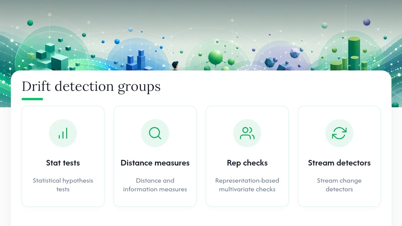
Detection approaches fall into four practical groups: statistical hypothesis tests, distance and information measures, representation-based multivariate checks, and stream change detectors. The right choice depends on label availability, data volume, and whether you are operating in batch or streaming mode.
Univariate statistical tests
The Kolmogorov–Smirnov (KS) test is the standard non-parametric method for comparing two continuous distributions. It measures the maximum absolute difference between two empirical cumulative distribution functions, producing a statistic and a p-value. It is sensitive, well-understood, and available in every major Python and R library. For categorical features, the chi-square test serves the same purpose by comparing observed versus expected frequencies across categories.
The Population Stability Index (PSI) is widely used in financial services because it produces a magnitude score rather than a binary reject/fail. PSI below 0.1 is generally considered stable, 0.1–0.2 warrants investigation, and above 0.2 signals significant shift. At large sample sizes, p-values from KS or chi-square tests become hypersensitive, flagging statistically significant but operationally trivial shifts. PSI and distance metrics sidestep this problem.
Distance and information measures
Wasserstein distance (also called Earth Mover’s Distance) measures the minimum cost of transforming one distribution into another. It is interpretable in the original feature’s units, which makes it useful for communicating drift magnitude to non-technical stakeholders. KL divergence and its symmetric variant JS divergence quantify the information difference between two distributions. Both are sensitive to zero-probability bins, so they require smoothing in practice. Maximum Mean Discrepancy (MMD) is a kernel-based measure that works well for high-dimensional or multivariate comparisons and is commonly used in representation drift monitoring for embeddings.
Stream and online change detectors
For streaming or near-real-time systems, batch statistical tests are too slow. Stream detectors such as DDM, EDDM, and ADWIN monitor error or statistic streams and trigger warnings or drift signals when recent behaviour statistically departs from earlier behaviour.
DDM (Drift Detection Method): Monitors the model’s error rate. When the error rate plus its standard deviation exceeds a threshold, DDM raises a warning; a further increase triggers a drift signal. Simple and effective for classification error streams.
EDDM (Early Drift Detection Method): An extension of DDM that is more sensitive to gradual drift by monitoring the distance between consecutive errors rather than the raw error rate.
ADWIN (Adaptive Windowing): Maintains an adaptive sliding window over a data stream and detects when the mean of a statistic in one sub-window differs significantly from another. Adaptive window methods are well-suited to streaming settings where the rate of change is unknown in advance.
KSWIN: A streaming variant of the KS test that applies the test within an adaptive window, combining the distributional sensitivity of KS with the online adaptability of ADWIN.
Page-Hinkley: A sequential analysis method that detects a persistent shift in the mean of a monitored variable. Computationally lightweight and well-suited to low-latency environments.
Pro Tip: At sample sizes above 50,000 observations per batch, p-values from KS and chi-square tests will flag almost every feature as drifted. Switch to PSI or Wasserstein distance as your primary signal, and use p-values only as a secondary filter.
How do you build a production-ready monitoring pipeline?
A monitoring pipeline has five components: a reference baseline, a windowing strategy, a sampling and aggregation layer, alerting rules, and operational integrations. Practical production monitoring requires baseline versioning, sliding or adaptive windows, sampling strategies, and clear alerting thresholds backed by runbooks.
Capture and version your reference baseline. The reference window should be a clean, representative slice of training data or the first stable weeks of production data. Version it alongside your model artefact so every drift report is reproducible. Refresh the reference when you retrain, not before.
Choose a window strategy. A fixed window compares each new batch against the static reference. A sliding window compares the most recent N observations against the reference, which is useful for detecting gradual drift. An adaptive window (as used by ADWIN) adjusts its size based on detected change, reducing latency for sudden shifts.
Define your sampling and aggregation approach. For high-volume systems, sample a statistically sufficient subset per batch rather than running tests on every record. For models serving multiple segments, run slice-level checks per country, product line, or customer cohort in addition to aggregate checks. A slice that drifts while the aggregate looks stable is one of the most common missed signals in enterprise deployments.
Set tiered alert thresholds. Combine three signals: the drift statistic for individual features, the feature’s importance rank in the model, and any measurable impact on model output distribution. A high-importance feature drifting beyond PSI 0.2 warrants immediate triage. A low-importance feature at PSI 0.15 warrants logging and review at the next scheduled check.
Integrate with your observability stack. Log every drift report to a time-series store (Prometheus, InfluxDB, or a data warehouse table). Surface results in a dashboard (Grafana, Looker, or a purpose-built ML observability tool). Attach each alert to a runbook that specifies the triage owner, the escalation path, and the decision criteria for retraining.
Pro Tip: Align each monitoring alert with a named business owner, not just a data science team member. When a fraud model’s input distribution shifts, the fraud operations lead needs to know as much as the ML engineer. This is particularly relevant for UK firms operating under FCA model risk expectations, where traceability of model change decisions is expected.
Which tools should you use for drift monitoring?
Tools such as Evidently, NannyML, River, MOA, and Frouros provide ready-made monitors for feature drift, streaming detectors, and in some cases label-free performance estimation. The right choice depends on your runtime, your label availability, and whether you need batch or streaming support.
Evidently: A Python library and open-source platform for batch drift monitoring. It generates HTML reports and JSON metrics for feature drift (KS, PSI, Wasserstein, chi-square), target drift, and data quality. Its report format integrates well with CI/CD pipelines and makes it straightforward to embed drift checks into scheduled jobs or model deployment gates. Best for teams running batch inference who want a fast, opinionated setup with minimal configuration.
NannyML: Distinguishes itself by offering confidence-based performance estimation without ground-truth labels, using a method called Confidence-Based Performance Estimation (CBPE). This is particularly valuable in production settings where labels arrive days or weeks after prediction. NannyML also provides univariate and multivariate drift detection. Best for classification models in settings with significant label delay, which is common in insurance claims, credit default, and fraud.
River: A Python library for online machine learning and streaming data. It implements ADWIN, KSWIN, DDM, EDDM, Page-Hinkley, and other stream detectors natively, alongside adaptive learning algorithms. MOA and River are frequently used in research and production for stream mining and adaptive learners. Best for real-time or near-real-time inference pipelines where batch checks introduce unacceptable latency.
MOA (Massive Online Analysis): A Java-based framework for stream mining, widely used in academic research and as a reference implementation for algorithms including ADWIN and EDDM. Less common in pure Python production stacks but valuable for teams working in JVM environments or needing access to a broad library of stream learning algorithms.
Frouros: A Python library focused specifically on drift detection, covering both batch and streaming scenarios. It implements a wide range of statistical tests and distance metrics (KS, MMD, Wasserstein, PSI, and others) with a consistent API. Frouros is particularly useful for teams that want a single library covering multiple detector families without pulling in a full ML observability platform.
For UK enterprise teams, Evidently and NannyML are the most production-ready options for batch monitoring, while River covers streaming needs. Frouros is a strong choice when you need fine-grained control over detector configuration without the overhead of a full platform.
How should you respond when drift is detected?
Detection is the easy part. The harder question is what to do next. Not every drift signal warrants retraining, and an undisciplined response to alerts is as costly as ignoring them.
Triage first. Before any model action, verify that the drift is real and not an artefact of a data pipeline failure. Check for upstream schema changes, missing values, or encoding errors. Slice the drift signal by time, geography, and product to understand whether it is broad or localised. A drift signal confined to a single data source or a single day is usually a pipeline issue, not a model issue.
Match the response to the drift type. The decision tree is roughly:
Schema or data quality issue: fix the pipeline, no model action required.
Prior/label drift with stable features: recalibrate the decision threshold, refresh the reference window.
Sustained covariate drift in high-importance features: selective retraining on recent data, or a full retrain if the shift is broad.
Confirmed concept drift: full retraining, or a switch to an online learning approach if labels arrive quickly enough.
Gradual drift across many features: consider an ensemble refresh or a model blend that weights recent data more heavily.
Deployment and validation discipline. Never deploy a retrained model directly to production. Use canary or blue-green deployment to route a small traffic fraction to the new model while the existing model continues serving the majority. Compare performance metrics between the two versions over a statistically meaningful window before promoting the new model. Maintain a rollback plan: the previous model artefact and its reference baseline should remain available for at least one full monitoring cycle after promotion.
Human-in-the-loop labelling is worth the investment for high-stakes decisions. In UK financial services, where model outputs affect credit decisions or fraud flags, a sample review process that generates fresh labels for ambiguous cases both improves retraining data quality and satisfies audit expectations for human oversight.
Pro Tip: Set a minimum drift duration threshold before triggering retraining. A single batch showing PSI above 0.2 may be noise. Two consecutive batches, or a sustained signal over 48 hours in a streaming system, is a more reliable trigger. This single rule eliminates the majority of unnecessary retrains.
How do you confirm that detected drift actually matters before retraining?
Drift in input distributions does not automatically mean model performance has degraded. Validating impact before committing to a retrain saves significant engineering time and avoids introducing instability from unnecessary model updates.
Metrics to monitor by task type
For classification models, track rolling AUC, precision, recall, and calibration (Brier score or reliability diagrams) over a sliding window. For regression models, monitor rolling MAE and RMSE. Calibration is particularly important for probabilistic outputs used in risk scoring: a model that ranks correctly but whose probabilities are systematically off will produce poor decisions at any fixed threshold.
Estimating impact without labels
When labels are delayed, use proxy signals. Score distribution shift (a change in the mean or variance of predicted probabilities) is a reliable early indicator that the model is behaving differently, even before outcomes are known. NannyML’s CBPE method formalises this by estimating performance from confidence scores alone. For regression, monitoring the distribution of residuals on a held-out validation set, refreshed periodically, provides a similar proxy.
Validation workflow before promoting a retrained model
Run the retrained model on a held-out acceptance test set drawn from recent production data. Confirm that performance metrics meet or exceed the thresholds defined in your model card.
Deploy via canary: route 5–10% of live traffic to the retrained model for a defined observation window (typically 24–72 hours for daily-batch systems).
Compare AUC, calibration, and business KPIs between the canary and the current model. If the canary underperforms on any primary metric, roll back immediately.
After full promotion, run a post-deployment check at 7 days and 30 days to confirm the retrained model is stable under current production conditions.
Validation step | What to check | Pass criterion |
Acceptance test | AUC, MAE/RMSE, calibration on recent holdout | Meets or exceeds baseline model thresholds |
Canary deployment | Live performance vs current model over 24–72 hours | No regression on primary business KPI |
Post-promotion check (7 days) | Score distribution stability, feature drift recurrence | PSI below 0.1 on top features |
Post-promotion check (30 days) | Rolling performance metrics, label-confirmed outcomes | Performance within agreed tolerance band |
How does a managed AI operations team run drift monitoring in practice?
The following describes the operational approach Sentient Concepts applies when running drift monitoring for UK enterprise deployments, covering the full cycle from baseline capture to retraining decision.
Baseline capture and model registration. At deployment, a versioned reference dataset is captured alongside the model artefact, training metadata, and a feature importance ranking. These are stored in a model registry with a linked data lineage record, which satisfies audit trail requirements for regulated UK firms.
Continuous monitoring layer. Batch inference jobs trigger a drift report on every run. The report covers univariate checks (KS, PSI) on the top 20 features by importance, a score distribution comparison, and a data quality summary (missingness, out-of-range values, schema conformance). For real-time inference systems, River-based stream detectors run inline and write drift events to a centralised log.

Alerting and triage. Alerts route to a shared incident channel with severity tags. Each alert links to a runbook specifying the triage owner (ML engineer for technical investigation, data science lead for model assessment, business owner for impact sign-off). The runbook includes a decision tree for the five most common drift scenarios encountered in that deployment.
Labelling pipeline and retraining cadence. Where labels are available, a labelling pipeline ingests ground-truth outcomes and computes rolling performance metrics. Retraining is scheduled on a defined cadence (typically monthly for stable models) with an out-of-cycle trigger if two consecutive monitoring runs breach the critical threshold. Post-retrain validation follows the canary workflow described above.
Operational roles:
ML engineer: Owns the monitoring pipeline, alert configuration, and data quality checks.
Data scientist: Interprets drift signals, decides on response strategy, and validates retrained models.
Platform/data engineer: Maintains the reference data store, logging infrastructure, and pipeline integrations.
Business owner: Signs off on retraining decisions for regulated models and reviews the audit trail.
Pro Tip: For UK firms under FCA or PRA oversight, attach a brief decision log to every retraining event: what drifted, when, what action was taken, and who approved it. This takes under ten minutes per event and provides the traceability regulators expect when they review model governance records. Aligning this with your AI change management process makes the governance overhead manageable.
The pragmatic rules of thumb for teams starting drift monitoring
Most teams starting drift monitoring make the same mistake: they try to monitor everything at once and end up with a dashboard full of alerts that nobody trusts. The more productive path is narrower and more deliberate.
Start with your top ten features by model importance and your model’s score distribution. These two checks will catch the majority of operationally significant drift events. Add data quality checks (missingness, out-of-range values) before you add any statistical test, because a missing value spike will produce a drift signal that looks like distribution shift but is actually a pipeline failure. Resolving the simpler problem first prevents wasted investigation time.
Prefer simpler detectors. KS and PSI are well-understood, easy to explain to stakeholders, and sufficient for most batch monitoring use cases. Escalate to MMD or multivariate two-sample tests only when you have evidence that univariate checks are missing genuine drift, which typically shows up as unexplained performance degradation without a clear univariate signal.
The organisational side matters as much as the technical side. A drift alert that lands in a team inbox with no owner, no runbook, and no defined escalation path will be ignored. Connecting monitoring alerts to business intelligence and competitive advantage requires that business owners understand what the alerts mean and what they are expected to do. That alignment is a design decision, not an afterthought. Build it before you go live, not after your first production incident.
For teams operating within an agile AI development lifecycle, drift monitoring fits naturally into the “operate” phase: it is the feedback loop that tells you when the “build” phase needs to restart. Treating it as a continuous process rather than a one-time deployment task is what separates teams that maintain model quality over time from those that discover degradation months after it began.
Sentient Concepts provides end-to-end drift monitoring and managed MLOps
Production drift monitoring is where many AI programmes stall. The statistical methods are well-documented, but operationalising them across regulated UK industries, with the right governance, tooling, and escalation paths, requires sustained engineering and operational discipline that most internal teams are not resourced to maintain alone.

Sentient Concepts delivers this as a managed service. The engagement typically begins with a readiness and data diligence assessment to establish what monitoring infrastructure exists, what reference data is available, and where the compliance gaps are. From there, the team designs and implements the monitoring pipeline through data and platform engineering, covering baseline versioning, alert configuration, logging, and dashboard integration. Ongoing drift monitoring, incident triage, and retraining decisions are then managed through Sentient Concepts’s managed AI operations service, with clear SLAs and audit-ready decision logs for regulated environments. To discuss how this applies to your current deployment, contact the team directly.
Sources
The following primary sources and project pages are the recommended starting points for deeper reading on drift detection methods, library documentation, and academic background.
FAQ
What is data drift detection?
Data drift detection is the process of continuously comparing the statistical distribution of input features in production against a reference baseline to identify when the data your model receives has changed significantly from the data it was trained on. It is the primary mechanism for catching model degradation before it affects business outcomes.
What is the difference between data drift and concept drift?
Data drift is a change in the distribution of input features P(X), while concept drift is a change in the relationship between inputs and the correct output P(Y|X). Data drift is often detectable without labels using statistical tests; concept drift requires labelled outcomes to confirm.
How often should you run drift monitoring in production?
For batch inference systems, run drift checks on every inference batch, typically daily or weekly depending on data volume. For streaming systems, use online detectors such as ADWIN or DDM that operate continuously. The monitoring frequency should match the cadence at which your model’s predictions affect decisions.
Which drift detection method works best for large datasets?
At large sample sizes, p-value-based tests such as the KS test become hypersensitive and flag operationally trivial shifts as significant. PSI and Wasserstein distance are more reliable for large datasets because they measure drift magnitude rather than statistical significance, giving you a stable signal regardless of sample size.
Can you detect drift without ground-truth labels?
Yes. Covariate drift, prior drift (via score distribution monitoring), schema drift, and embedding drift are all detectable without labels. Tools such as NannyML extend this further by estimating model performance from prediction confidence scores alone, using its CBPE method, which is particularly useful when labels are delayed by days or weeks.
Recommended