Book Capacity 12 Weeks Out: Lane Level Demand Forecasting for Logistics
Demand forecasting in logistics predicts shipment and inventory volume by lane, mode, and time horizon, giving planners enough lead time to commit capacity instead of buying it at spot-market prices. The operational payoff is straightforward: freight booked weeks ahead costs less and disrupts fewer schedules than freight booked in a panic. This guide covers the methods, implementation steps, accuracy benchmarks, and the growing role of machine learning in getting forecasts right.
TL;DR:
Accurate demand forecasting at lane level enables logistics teams to lock in capacity early and avoid spot-market premiums, especially within 8 to 12 weeks of execution.
Combining historical shipment data with external indicators like retail sales or PMI improves forecast reliability, but models must be tailored to specific horizons and demand volatility.
Implementing a continuous ownership process with operational input and system integration ensures forecasts are trusted and consistently used in decision-making.
Using simple time-series models as a baseline, layered with causal variables or machine learning where data density allows, optimizes forecast accuracy without unnecessary complexity.
Setting clear forecast objectives, validation criteria, and rollback plans during short pilots minimizes organizational risk and accelerates deployment success.
Table of Contents
Why demand forecasting matters for logistics: benefits, failure modes, and lead time
Data inputs, leading indicators, and realistic accuracy targets
Case evidence: what an end-to-end approach delivers in practice
Integration of demand forecasting with supply chain and inventory management systems
Risk management and scenario planning using demand forecasts
What separates forecasting programmes that work from those that don’t
Where Sentient Concepts fits if you want a partner to run it
What demand forecasting means in a logistics context
Demand forecasting produces a number: expected volume, by lane, customer, or cargo type, over a defined horizon. In logistics, that number has to be granular enough to drive a decision, not just a boardroom chart. A forwarder forecasting 500 TEU on a transpacific lane next quarter needs that figure broken down by origin port and customer tier, because the contracting decision depends on it.
Forecasting and demand planning are related but not the same discipline. Forecasting generates the predictive number; demand planning turns that number into commitments, capacity bookings, staffing rosters, and inventory targets. ASCM’s guidance on demand and supply planning stresses that the two functions must run together, using historical sales, known events, and statistical methods alongside cross-functional input, or the forecast becomes an academic exercise nobody acts on.
Ownership typically splits three ways:
Operations teams run the forecasting models and own the horizon assumptions.
Commercial and sales teams supply pipeline visibility and customer booking intent that models cannot see on their own.
Finance and procurement consume the output to set contracting budgets and capacity commitments.
Miss any one of these voices and the forecast drifts from reality. Sales teams often know about a customer’s expansion plans months before that demand shows up in historical shipment data, and a model trained purely on the past will always be the last to know.
Why demand forecasting matters for logistics: benefits, failure modes, and lead time
Forecasting accuracy translates directly into freight spend. Book capacity 12 weeks out and you negotiate contract rates; book it 12 days out and you pay spot-market premiums, often with no guarantee of space at all. The GoFreight analysis of forwarder forecasting makes the point plainly: forwarders who forecast by trade lane and horizon can commit carrier capacity, schedule labour, and set quoting strategy with confidence, rather than reacting to bookings as they land.
The benefits compound across the operation:
Lower freight spend through contracted rather than spot capacity.
Better roster planning at warehouses and terminals, avoiding overtime spikes.
Improved on-time-in-full (OTIF) performance because capacity is secured before it is needed.
Fewer detention and demurrage charges from containers sitting idle while capacity gets sorted out late.
Get forecasting wrong and the costs show up fast: expediting fees, blown budgets, and the bullwhip effect, where small demand fluctuations at the retail end amplify into wild swings further up the chain. CIPS identifies demand forecasting as the primary lever for controlling bullwhip, because aligning manufacturing and logistics planning with actual end-user order patterns stops the amplification at source.
Pro Tip: Map every forecast horizon to the specific decision it unlocks. A forecast that doesn’t change a booking, a hire, or a contract term is just a number on a dashboard.
Forecasting methods and how to choose between them
No single method fits every lane, product, or data situation. Choosing correctly comes down to three questions: how much historical data exists, how volatile the demand pattern is, and how far ahead the decision needs visibility.
Time-series methods (exponential smoothing, ARIMA) work well on stable, established lanes with several years of clean historical volume. They’re computationally cheap, easy to explain to a commercial director, and often accurate enough for mature trade routes where demand moves in recognisable seasonal rhythms.
Causal and regression methods earn their place when an external variable drives volume more than history does. If freight volume tracks a customer’s retail sell-through or a manufacturing index, a regression model that incorporates that variable will outperform a model that only looks backwards.
Machine learning approaches (gradient boosting, ensemble methods) justify their added complexity once you have enough data density, typically multiple years of weekly observations across several correlated lanes, and once accuracy gains actually matter financially. ML tends to shine when it can absorb leading indicators that simpler models can’t handle: web search trends, purchasing manager indices, or competitor capacity announcements.
Qualitative methods (sales input, expert judgement, analogous-lane comparison) are the only sensible option for new lanes or new products with no historical trail. A model trained on nothing produces confident nonsense; a commercial team with market knowledge produces a usable estimate.
Hybrid approaches blend a statistical baseline with a qualitative overlay, letting planners adjust the model’s output when they know something the data doesn’t. This is standard practice, not a compromise. SAP’s guidance on modern demand forecasting points out that even mature forecasting programmes rely on this blend, because no algorithm captures a customer’s phone call announcing a factory relocation.
Most logistics teams should start with a time-series baseline, layer in causal variables where they exist, and reserve full ML deployment for the highest-volume lanes where the accuracy gain pays for the added complexity.
A five-step process for implementing demand forecasting
Getting from spreadsheet guesswork to a working forecasting programme follows a fairly consistent sequence across logistics organisations, regardless of size.
Align on objectives and horizons. Before touching any data, agree with operations, commercial, and finance stakeholders what decisions the forecast needs to support and over what horizon. A forecast built for a 52-week sales plan looks nothing like one built for 4-week staffing decisions, and building one model to serve both purposes usually satisfies neither.
Collect and prepare data. Pull historical shipment volumes, booking data, and customer order patterns, then layer in leading indicators where they exist. Data quality matters more than model sophistication at this stage; a clean three-year history beats a messy five-year one every time.
Build a baseline and select additional models. Start with a simple time-series baseline for each lane, then test whether causal variables or leading indicators materially improve on it. The 2024 literature review on logistics demand forecasting found that simple aggregation heuristics often remain competitive with more complex methods, so resist the urge to add complexity before proving the baseline is actually inadequate.
Validate and backtest. Run the model against known historical periods it hasn’t seen and set lane-level accuracy targets before going live. Define what “good enough” looks like in advance, because arguing about acceptable error bands after a bad forecast has already cost money is a conversation nobody wins.
Hand off into operations. Feed forecast output into sales and operations planning (S&OP), capacity contracting cycles, and workforce rostering. A forecast that lives in a report nobody reads has delivered zero value, no matter how accurate it was.
Data inputs, leading indicators, and realistic accuracy targets
Forecasting quality depends heavily on what goes into the model. Core internal data includes historical shipment volumes, booking lead times, customer order patterns, and cancellation rates. External leading indicators add real predictive power: point-of-sale data from major retail customers, web search trend data for consumer goods, purchasing manager indices (PMI) for manufacturing-linked freight, seasonal weather patterns, and carrier sailing schedules.
Different horizons serve different decisions, and conflating them is one of the most common planning mistakes.
Horizon | Typical decision | Primary data inputs |
4 weeks | Warehouse and terminal staffing rosters | Recent bookings, short-term order patterns |
8 to 12 weeks | Carrier capacity commitments | Historical volume, customer pipeline, PMI |
12 to 26 weeks | Contract negotiation window | Seasonal patterns, contract renewal cycles |
52 weeks | Annual sales and network planning | Full historical trend, strategic account plans |
Accuracy expectations should be scoped to the horizon and lane maturity, not treated as a single universal number. Mean Absolute Percentage Error (MAPE) is the standard metric, but the “good” range varies enormously: mature, high-volume lanes with stable customers often land in the 10 to 20% MAPE range at a 4 to 8 week horizon, while new lanes, volatile commodities, or 52-week horizons routinely sit above 30% and still deliver planning value. Bias (whether a model consistently over- or under-forecasts) matters as much as raw error, because a model that’s wrong in a consistent direction is easier to correct than one that’s randomly wrong.
How AI and machine learning change forecasting outcomes
Machine learning earns its place in logistics forecasting where the problem outgrows what a spreadsheet or a simple statistical model can handle: cross-correlated lanes, high-frequency leading indicators, and hierarchies that need to stay internally consistent (a corridor total that doesn’t match the sum of its lane-level forecasts is a credibility problem, not a rounding error).
Model choice should follow the horizon, not the hype:
For tactical decisions inside a 1 to 4 week window, gradient boosting models such as XGBoost or LightGBM tend to outperform deep learning approaches while needing far less data and compute.
For longer horizons where structural seasonality matters more than short-term noise, architectures like Prophet or N-BEATS capture recurring patterns that boosting models can miss.
Ensembles that combine several model families tend to be more robust than any single model, particularly across lanes with different volatility profiles.
Practitioner reporting on AI-driven logistics forecasting notes that leading indicators such as point-of-sale data, web search volume, and PMI readings, combined with hierarchical models that reconcile lane-level and corridor-level totals, meaningfully improve responsiveness over models trained on shipment history alone.
The pitfalls are just as real as the upside. Insufficient historical data produces overconfident, unreliable models. Overfitting to noise in a volatile lane creates forecasts that look precise and perform badly. And organisational adoption often fails not because the model is wrong, but because the team that has to act on it was never consulted while it was built.
Pro Tip: Never deploy a model more complex than your team can explain to the person who has to defend the resulting decision to a customer.
Lane-level considerations for freight forwarders
Forwarders should forecast at lane level and preserve the house bill to master bill linkage, because aggregate corridor numbers hide the load factor problems that actually cost money. A corridor might look healthy on paper while individual lanes run under capacity, quietly eating margin.
Track load factor by lane, not just total volume, to catch underutilisation before it shows up in a quarterly review.
Use agent and destination-side booking signals to extend effective lead time; a destination agent often sees demand building before it reaches the origin booking system.
Apply a structured peak-season lookback: GoFreight’s approach to lane-level forecasting recommends using two to three years of weekly TEU data by lane, normalised to a peak-week index, to build a defensible ramp curve for the busy season.
Adjust for known calendar events. Retailer promotional calendars and Lunar New Year timing shift demand in ways that pure historical averaging will always get wrong if the event date moves year to year.
Case evidence: what an end-to-end approach delivers in practice
The gap between a forecasting pilot that works in a spreadsheet and one that runs reliably in production is usually organisational, not mathematical. Handoffs between the team that builds the model and the team that has to operate it are where most forecasting programmes quietly stall.
Some AI firms work across finance, manufacturing, and logistics on this handoff problem, building AI systems and then maintaining them rather than delivering a model and walking away. Relevant work includes automating Bill of Lading generation, where document automation reduced the manual processing steps sitting between a booking and an operational shipment record, and supplier document processing automation in manufacturing settings, where reducing document handling time freed planning staff to focus on demand-side decisions rather than paperwork.
Continuity of ownership from strategy through to ongoing operation avoids the “model built, then abandoned” pattern common with pilot-only engagements.
Document automation adjacent to forecasting reduces the manual data-entry lag that corrupts leading-indicator accuracy.
Tailored deployment across finance, manufacturing, and logistics shows the underlying approach transfers across sectors with different data maturity.
Reducing the handoffs between strategy, engineering, and operations is what turns a forecasting model from a one-off analysis into something a logistics team can actually run week after week.
A 90-day pilot plan you can run now
A forecasting pilot doesn’t need six months to prove its worth. Ninety days is enough to validate whether the approach earns wider rollout.
Weeks 1 to 2: Pick two or three lanes with clean historical data and real operational pain, such as recurring capacity shortfalls or spot-buying spikes.
Weeks 3 to 4: Prepare and clean the historical data, and identify one or two leading indicators worth testing.
Weeks 5 to 8: Build a statistical baseline and one machine learning model, then backtest both against a held-out historical period.
Weeks 9 to 10: Set a MAPE target scoped to the horizon and lane maturity, and agree it with operations before going live.
Weeks 11 to 13: Run the forecast live alongside existing planning, with a weekly feedback loop comparing forecast to actual.
Governance matters as much as the model. Set a fixed review cadence (weekly during the pilot), name who has authority to act on the forecast, and agree rollback criteria in advance: if accuracy misses target for two consecutive cycles, the team reverts to the previous planning method rather than persisting with a model that isn’t earning its keep.
Pro Tip: Write down your rollback criteria before the pilot starts, not after a bad forecast makes the decision emotional.
If the pilot clears its MAPE target and the operations team finds the output genuinely useful, the next step is extending the same approach to more lanes and integrating it into the standing S&OP cycle.
Integration of demand forecasting with supply chain and inventory management systems
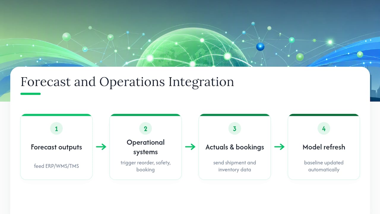
A forecast that stays in a standalone spreadsheet delivers a fraction of its potential value. The real payoff comes when forecast output flows directly into the systems that translate a number into action: enterprise resource planning (ERP), warehouse management systems (WMS), and transport management systems (TMS).
Practically, this means the forecast needs to feed reorder point calculations, safety stock policies, and capacity booking workflows automatically, rather than requiring a planner to manually re-key numbers between systems every week. Coursera’s primer on inventory management explains how forecast outputs link directly to reorder points and min/max inventory policies, and that link breaks the moment a human has to bridge two disconnected systems by hand.
Integration also needs to run in the other direction. Actual shipment data, booking confirmations, and inventory drawdowns should feed back into the forecasting model automatically, so the baseline stays current without a manual data refresh cycle. Systems that only push forecast data outward but never pull actuals back in tend to drift out of sync within a few months.
For teams weighing how to connect a forecasting model to existing ERP and TMS infrastructure, the technical integration work is often the harder half of the project, harder than building the model itself. FlowLab’s guidance on ERP integration covers the practical approach to connecting planning outputs with operational systems, which is worth reviewing before committing to a forecasting platform that can’t talk to what you already run.
Handling seasonality and trend changes in logistics demand
Logistics demand carries two distinct seasonal patterns that get conflated far too often: calendar seasonality (Lunar New Year, Christmas retail peaks, harvest cycles) and structural trend shifts (a customer permanently moving volume to a new lane, a modal shift from air to ocean).
Calendar seasonality is predictable but not fixed. Lunar New Year moves by weeks each year on the Western calendar, and a model that naively averages “week 6 of the year” across multiple years will systematically misjudge the ramp. The fix is normalising historical data to the event date itself, not the calendar week, then reapplying the correct calendar date for the forecast year.
Trend changes are harder because they don’t announce themselves in clean historical patterns. This is exactly where qualitative input from commercial teams earns its keep: sales conversations often reveal a structural shift long before enough data points exist to let a statistical model detect it on its own.
The practical approach is to run two views side by side: a statistical model tracking the recent trend line, and a qualitative overlay capturing known account-level changes. When the two disagree significantly, that’s the signal worth a planning meeting, not a reason to trust one over the other by default.
Risk management and scenario planning using demand forecasts
A single-point forecast, one number for next quarter’s volume, hides the range of outcomes that could actually happen. Scenario planning turns that single number into a working risk management tool by modelling a small set of plausible futures instead of pretending certainty exists where it doesn’t.
A practical scenario set for most logistics operations includes three cases: a base case built from the primary forecast model, an upside case reflecting stronger-than-expected demand or a competitor’s capacity exit, and a downside case reflecting demand softening or a disruption event (port congestion, a carrier alliance restructuring, a regional shutdown). Each scenario should carry its own capacity and staffing implication, not just a different volume number.
The value shows up when disruption actually hits. The 2024 literature review on logistics demand forecasting points out that coordination across supply chain echelons matters more than model sophistication when disruption hits, because a forecast that’s accurate at the lane level but disconnected from upstream supplier or downstream customer behaviour still leaves the organisation exposed.
Scenario planning works best as a standing quarterly exercise tied to the 12 to 26 week contracting horizon, not a one-off exercise pulled out only when a crisis is already underway. By the time disruption is visible in the data, the window for a planned response has usually already closed.
What separates forecasting programmes that work from those that don’t
The most common failure isn’t a bad model. It’s a good model nobody trusts enough to act on, because the team running operations was never involved in building it. A forecast that arrives from a separate analytics function with no channel for operational feedback gets quietly overridden within a few cycles, and the whole investment stalls.
The fix is straightforward but rarely followed: treat the model build and the operational rollout as one continuous project with shared ownership, not a handoff from data science to operations. Forecasting programmes that stick are the ones where the operations manager who has to defend a booking decision to a customer helped set the accuracy target in the first place, rather than inheriting one from a report they never saw drafted.
Integrating the model with day-to-day decision making matters more than any algorithm choice discussed earlier in this piece. A mediocre model that operations trusts and acts on consistently will outperform an excellent model that sits in a dashboard nobody opens.
— Thomas Samuel
Where Sentient Concepts fits if you want a partner to run it
Building a forecasting pilot in a spreadsheet is one thing; running it reliably across dozens of lanes, integrated with your TMS and WMS, with someone accountable when the model drifts, is another problem entirely. Closing the gap between strategy, engineering, and ongoing operation with one accountable team, without the handoff between “the people who built it” and “the people who have to keep it running,” is a critical factor in successful forecasting projects.
The typical path runs from a scoped pilot on two or three priority lanes, through deployment integrated with existing planning systems, into managed AI operations that keep the model monitored, retrained, and accountable to someone rather than left to drift. Sentient Concepts’ supply chain and logistics practice covers exactly this kind of engagement, from forecasting model build through to the operational systems that act on its output.
If your team has the lanes and pain points identified but lacks the bandwidth to build, integrate, and maintain a forecasting system in-house, it may be worthwhile to consult with specialists to scope a pilot against the 90-day plan outlined above.
Sources
FAQ
What are the five main types of demand forecasting methods?
The five main approaches are time-series methods (exponential smoothing, ARIMA), causal or regression methods, machine learning models (gradient boosting, ensembles), qualitative methods for new lanes or products, and hybrid approaches that blend a statistical baseline with human judgement.
What is demand forecasting in logistics?
Demand forecasting in logistics predicts shipment or inventory volume by lane, mode, and time horizon, giving planners enough lead time to book capacity and staff operations ahead of need rather than reacting to demand as it arrives.
How do you forecast supply and demand together?
Effective forecasting combines historical volume data and statistical methods with supply-side input on capacity, contracts, and known events, coordinated across sales, operations, and finance rather than run as a standalone analytics exercise.
What are the 5 P’s of logistics?
Definitions of the “5 P’s” vary by source and aren’t a single standardised industry framework; most common versions reference product, price, promotion, place, and people, though logistics practitioners more consistently rely on horizon-based planning (4, 12, 26, and 52-week decisions) than this looser marketing-derived list.
How accurate should a logistics demand forecast be?
Accuracy expectations depend on lane maturity and horizon: mature, high-volume lanes at a 4 to 8 week horizon often achieve a MAPE of 10 to 20%, while new lanes or 52-week horizons commonly exceed 30% and still deliver useful planning value.
Recommended